Upgrade to Microsoft 365 to work anywhere with the latest features and updates. Due to changes with how windows are containerized in Excel 2013 and later you no longer protect Windows in those versions when protecting a workbook.
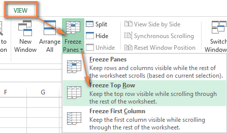
How To Freeze Panes In Excel Lock Rows And Columns
You can freeze a pane that contains multiple rows or multiple columnsor even freeze a group of columns and a group of rows at the same time.

Freeze panes excel 2013. Divide Page Into Columns. You can also use panes to freeze headings in the top rows and first columns so that the headings stay in view at all times no matter how you scroll through the worksheet. The next step is to go back to Freeze Panes and choose Freeze Panes this time instead of Freeze Top Row.
If you are working with Excel for Mac 2011 then read this article instead. This article isnt a detail discussion on what events are or their features. To freeze the top row execute the following steps.
Unfreeze rows or columns 492 People Used More Information Visit Site How to freeze a row in Excel so it always stays visible. Click the row number at the left side of the spreadsheet. Open a spreadsheet in which you wish to freeze a pane.
This will now freeze all the rows above row 6. Enter your email. How to Add a PDF to Excel.
In Excel freeze panes to compare information and use view options in Excel to more easily read Excel spreadsheets. To lock rows select the row below where you want the split to appear To lock columns select the column to the. We use three rows merely as an example.
Shade Every Other Row. I am successfully able to freeze the top row. Freeze Top Row.
Excel 365 2016 2013 2010 2007 2003. Youre scrolling down your worksheet or scrolling to the side but part of it is frozen in place. Through VBA we can control what happens at certain events such as before printing or.
Heres the first spreadsheet well be messing with. Excel for Microsoft 365 Excel for the web Excel 2019 Excel 2016 Excel 2013 Excel 2010 Excel 2007 More. Excel lets you freeze things in one of three ways.
Freeze rows or columns. Work anywhere from any device with Microsoft 365. Excel 2013 - Freezing Panes and View Options.
Click Freeze Top Row. The steps in this guide will show you how to freeze the top three rows of a spreadsheet in Excel 2013. You can freeze a row in Excel so its easier to compare data as you scroll through the spreadsheet.
If the Windows option for the Workbook Protection is enabled then it will make your Excel Freeze Panes not working. This tutorial will walk you through how to freeze panes in Excel 2013. Instructions in this article apply to Excel 2019 2016 2013 2010 2007.
Panes are great for viewing different parts of the same worksheet that normally cant be seen together in Excel 2013. Excel Calculations Are Wrong. You can freeze the top row.
On the View tab in the Window group click Freeze Panes. Scroll down to the rest of the worksheet. Tap to the Review tab from the Excel ribbon.
Freeze the Top Row of a Worksheet Freezing the top row of a worksheet is a great way to keep your Excel headings visible at all times. What Excel version do you use. Freeze Panes will freeze all columns to the left of your selected column.
Apply for a job. However each time I open the spreadsheet I have to manually re-freeze the top row. And Excel for Mac 2016 and later.
As shown in Figure 3 the Windows command is permanently disabled in Excel 2013 and later. Select View Freeze Panes Freeze Panes. This same process can be applied to any number of the top rows in your spreadsheet.
To fix this click View Window Unfreeze Panes. You can freeze the leftmost column. Is there any way to permanently freeze the top row so I do not have to do.
In this spreadsheet you want to see the first three columns and last column in one frame since you want to know the net salary each employee is receiving. On the worksheet do one of the following. September 25 2020.
In the screenshot above we simply zoomed out to see the entire spreadsheet. I do so and then save. Instead it gives an example of a WorkBook Event.
This is probably because at some point you decided to freeze the panes. To freeze row or column headings or both follow these steps. Fix Excel Freezing or Slow.
To keep an area of a worksheet visible while you scroll to another area of the worksheet go to the View tab where you can Freeze Panes to lock specific rows and columns in place or you can Split panes to create separate windows of the same worksheet. To enable the Freeze Panes option again you need to unprotect your Excel workbook. This way you can keep rows or columns visible while scrolling through the rest of the worksheet.
Word 2016 2013. March 12 2015 at 1208 pm. Freeze the Top Row.
Force Workbook to Save Without Freeze Panes. In Excel 2013 and 2010 the Freeze Panes button is on the View tab. Now you can scroll through the data while the four rows of data for StandID 1001 Year 2013 and ProductID A10011 remain visible.
These are events that are held at the workbook level rather than a particular worksheet. Open your spreadsheet in Excel 2013. Improve my work skills.
The save will not stick. Excel lets us control things through events. Well this Windows option seems permanently disabled in Excel 2016 and 2013.
Get started with computers. You can freeze your column and row labels so that you can view them no matter how far you scroll down or to the right in your worksheet. If you have a large table of data in Excel it can be useful to freeze rows or columns.
So lets take a look at how to perform these actions. Excels Freeze Panes command also becomes disabled when the workbook is protected in Excel 2010 and earlier as illustrated in Figure 2. You can choose to only freeze the first visible row in your Excel sheet or freeze.
Excel 2016 Excel 2019 Office 365.
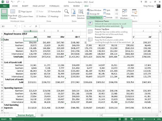
How To Freeze Panes In Excel 2013 Dummies
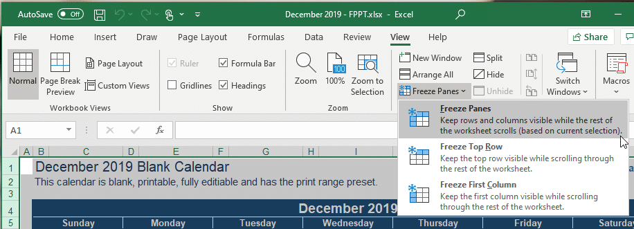
How To Freeze Panes To Lock Columns And Rows In Excel
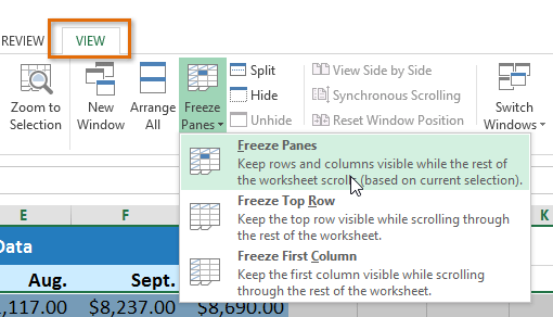
Excel 2013 Freezing Panes And View Options
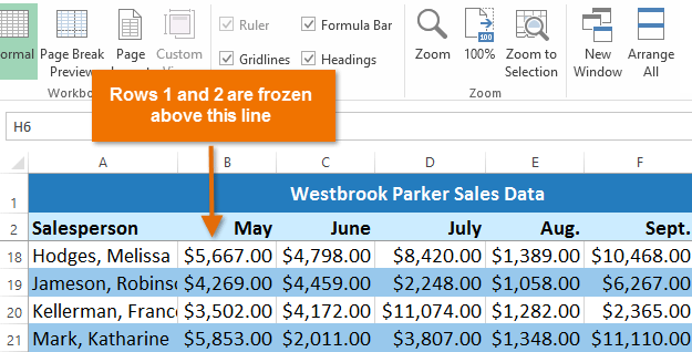
Excel 2013 Freezing Panes And View Options

How To Freeze Lock Rows And Columns In Excel Bettercloud Monitor