With conditional formatting cells can be formatted in different colours schemes. Over 30 examples of formulas you can use to apply conditional formatting to highlight cells that meet specific criteria with screen shots and links to full explanations.
Use Conditional Formatting To Highlight Information Excel
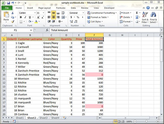
Suppose you want to find cell with Amount 0 and Mark them as redChoose.

Excel 2010 conditional formatting. How to Use Conditional Formatting. Format only values that are above or below average - Applies conditional formatting to cells falling above or below the average as calculated by Excel. Format only unique or duplicate values - Applies conditional formatting to either unique or duplicate values.
Enter a formula that returns TRUE or FALSE. Enter the value 60 and select any formatting style. The conditional formatting rules for the current selection are displayed including the rule type the format the range of cells the rule applies to and the Stop If True setting.
Its for an earlier version of Excel but the interface really hasnt changed much. What conditional formatting aims to achieve is to give you a visual way of representing your data that is more easy to take in and understand than merely presenting numbers in a spreadsheet. If you are using the example apply formatting to all of the sales data.
MS Excel 2010 Conditional Formatting feature enables you to format a range of values so that the values outside certain limits are automatically formatted. Formulas that apply conditional formatting must evaluate to TRUE or FALSE. Instructions apply to Excel 2019 2016 2013 2010.
On the Home tab in the Styles group click Conditional Formatting. Excel 2010s conditional formatting lets you change the appearance of a cell based on its value or another cells value. Navigate to Home tab and click Conditional Formatting button you will see list of different options.
Open an existing Excel 2010 workbook. Apply conditional formatting to a range of cells with numerical values. Take your Excel skills to the next level and use a formula to determine which cells to format.
Set formatting options and save the rule. Excel 2010s conditional formatting feature lets you reference different sheetssomething you couldnt do before. This is especially useful if you have applied multiple rules to the cells.
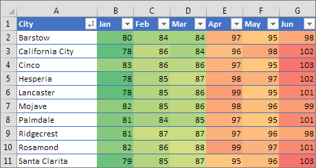
You might use conditional formatting to locate dates that meet a certain criteria such as falling on a Saturday or Sunday to call out the highest or lowest values in a range or to indicate values that fall under over or between specified amounts. Select the Marks column go to conditional formatting and in Highlight Cells Rules click Less than. This type of formatting lets you visualise large and complex data sets allowing you to spot data trends and missing data more easily and quickly.
The ISODD function only returns TRUE for odd numbers triggering the rule. To make conditional formatting easier Excel supports pre-set options that cover commonly used situations such as. This Excel tutorial explains how to use conditional formatting to change the fill color of a cell based on the value of another cell in Excel 2010 with screenshots and step-by-step instructions.
Rather than this formatting being applied to all cells in a range it is applied selectively and. Conditional Formatting with Formulas. Normally the data can be visually differentiated using one or more rules however in this article we will discuss how to apply conditional formatting with 2 conditions.
Using Conditional Cell Formatting in Excel 2007. The cells to be distinguished depend on pre-specified fixed conditionsThe advantage of conditional formatting which is used across a. Microsoft Excel 2010 provides a variation on formatting known as conditional formatting.
Use a formula to determine which cells to format - Applies conditional formatting to. To apply conditional formatting in Excel 2010 select the cells you want to analyse and then click Home Styles Conditional Formatting. In Microsoft Excel 2010 Im trying to apply a fill color to a cell based on the value in an adjacent cell.
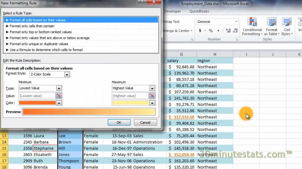
Create a conditional formatting rule and select the Formula option. If youve never used Conditional Formatting before you might want to look at Using Conditional Cell Formatting in Excel 2007. If you want you can use this example.
Select the range A1E5. How to apply conditional formatting with a formula. You specify certain conditions and when those conditions are met Excel applies the formatting that you choose.
Choose Home Tab Style group Conditional Formatting dropdown. This article explains five different ways to use conditional formatting in Excel. Excel for Mac Excel for Microsoft 365 and Excel Online.
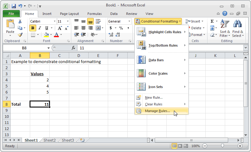
The conditional formatting is used to create visual differentiation in a large set of data in some standard format. The Conditional Formatting Rules Manager dialog box appears. In earlier versions you had to copy or link data to the same sheet.
That guide talks about formatting specific cells based on their content. On the Home tab in the Styles group click the arrow next to Conditional Formatting and then click Manage Rules. Since Microsoft 2007 Excel the popular spreadsheet processing software has included conditional formatting.
Select the cells you want to format. You can edit or delete individual rules by clicking the Conditional Formatting command and selecting Manage Rules.

Three Tips For Using Excel S Conditional Formatting More Efficiently Techrepublic
Conditional Format In Excel 2010 Tutorialspoint
Ms Excel 2010 Change The Font Color Based On The Value In The Cell
Excel 2010 Conditional Formatting Formulas Youtube
![]()
Conditional Formatting In Excel 2007 And 2010 Spreadsheets Using Formulas And Icon Sets Turbofuture Technology